Linear Combinations and the Multiple Comparison Problem

Objectives

Recognize the limitations of the alternative hypothesis in an ANOVA F-test.
Construct and interpret linear combinations of group means.
Understand the need for multiple comparison procedures and when to apply them.
Apply methods such as Bonferroni and Dunnett to test planned and unplanned comparisons.

Fallacies in Hypothesis Testing

False causality: A small p-value does not indicate causation. Causality can only be inferred from randomized experiments, not observational studies.
Accepting the null: We should say there is “no evidence of a difference,” not that the null hypothesis is true. There is not enough evidence to suggest the observed difference is due to anything other than chance.
Statistical vs. practical significance: Statistical significance does not imply practical importance. Evaluate practical significance using power, effect size, and confidence intervals.
- Differences that are statistically but not practically significant may arise due to large sample sizes.
- If a difference is practically significant but not statistically significant, more data may be needed.
Data dredging: Avoid fishing for significance (data snooping). This can lead to publication bias against negative results.
Good statistics from bad data: Biased or non-random data compromise conclusions. Experimental design determines which inferences and statistical methods are valid.

Linear Combination of Group Means

ANOVA allows only pairwise comparisons of means and does not account for meaningful structure across groups. In practice, you may wish to compare the average of several means to a single group, or to the average of others.
The ANOVA F-test serves as an initial screening tool for detecting any overall differences in means. If the F-test is significant, follow-up tests can be considered.

Linear Contrasts

A linear combination of group means is defined as: \[ \gamma = C_1\mu_1 + C_2\mu_2 + \dots + C_I\mu_I \] where $\gamma$ represents the linear combination and the $C_i$ are coefficients. When the coefficients sum to zero, the combination is called a contrast.
Estimate $\gamma$ using $g = C_1\bar{x}_1 + C_2\bar{x}_2 + \dots + C_I\bar{x}_I$, where $\bar{x}_i$ are group sample means.
The standard error of $g$, denoted $SE(g)$, is given by: \[ SE(g) = S_p \sqrt{\frac{C_1^2}{n_1} + \frac{C_2^2}{n_2} + \dots + \frac{C_I^2}{n_I}} \] where $S_p$ is the pooled standard deviation.
Even when comparing only two groups (i.e., the other coefficients and terms under the square root are zero), the pooled standard deviation is used under the assumption of equal variances across all groups.
The t-statistic for testing contrasts is: \[ t_{\alpha, df} = \frac{g - \gamma}{SE(g)} \] where $g$ is the observed linear combination, $\gamma$ is the hypothesized value (e.g., $\gamma = 0$), and $df$ is the degrees of freedom associated with $S_p$.

Steps for a Linear Contrast Test

Summarize the data: Obtain group means, sample sizes, and the pooled standard deviation from the ANOVA model (e.g., RMSE).
Specify the coefficients: Choose $C_i$ values such that $\sum C_i = 0$.
Estimate the contrast: Compute the linear combination $g$ using the sample means and chosen coefficients.
Compute the standard error: Calculate $SE(g)$ using the formula above.
Construct confidence intervals: \[ CI = g \pm t_{\alpha, df} \cdot SE(g) \]
Perform the test: Calculate the t-statistic to assess the contrast.

Simultaneous Inferences

When testing multiple contrasts or pairwise comparisons, the risk of a Type I error increases. Adjustments to significance levels or p-values are needed to maintain the overall error rate.
Distinguish between:
- Individual confidence level: The probability that a single interval captures its parameter ($1 - \alpha$).
- Familywise confidence level: The probability that all intervals simultaneously capture their parameters. This probability is less than $1 - \alpha$ unless corrections are applied.

Common Applications of Linear Contrasts

Comparing average values, e.g., the mean of groups 1 and 2 versus group 3.
Comparing response rates across treatments, such as dietary interventions in animals.
Testing specific hypotheses about structured combinations of group means.

Adjusting for Multiple Comparisons

When conducting multiple tests, it is important to control the familywise error rate (FWER). Common post-hoc procedures are outlined below.

Procedures for All Pairwise Differences in Means

Bonferroni adjustment
- Adjusts the significance level: \[ \text{Adjusted } \alpha = \frac{\alpha}{\# \text{ comparisons}} \]
- Example: For 4 groups, there are $\binom{4}{2} = 6$ pairwise comparisons (i.e., 4 choose 2): \[ \alpha' = \frac{0.05}{6} = 0.0083 \]
- Strengths: Simple, widely applicable
- Weaknesses: Very conservative; reduces power
Tukey’s Honestly Significant Difference (HSD)
- Used to construct simultaneous confidence intervals for all pairwise mean differences
- Based on the studentized range statistic: \[ q = \frac{\bar{X}_{\text{largest}} - \bar{X}_{\text{smallest}}}{\sqrt{\frac{MSE}{n}}} \] (for groups with equal $n$)
- Confidence intervals: \[ (\bar{X}_i - \bar{X}_j) \pm q_{\alpha, (k, N-k)} \cdot \sqrt{\frac{MSE}{n}} \]
  - When group sizes are unequal, use the harmonic mean of $n_i$ and $n_j$ (as done in SAS): \[ n_{ij} = \frac{2 \cdot n_i \cdot n_j}{n_i + n_j} \]
- Strengths: Maintains FWER; easy to interpret
- Weaknesses: Assumes equal variances (can be extended via Tukey-Kramer)
Ryan-Elliot-Gabriel-Welsch Q (REGWQ) procedure
- Recommended by SAS; balances power and Type I error control
- Method:
  1. Order the group means in descending order
  2. Reject $H_0$ if: \[ \text{Difference} > q_{\text{critical}} \cdot \text{Studentized range} \]
  3. Adjust the p-values for the number of comparisons
- Strengths: High power; nominal Type I error
- Weaknesses: Algorithmically complex

Procedures for Pairwise Differences vs. Control

Dunnett’s procedure
- Compares each treatment group to a single control group
- Uses the $D$-statistic: \[ D = d_{(k-1, N-k)} \cdot \sqrt{\frac{2 \cdot MSE}{n_{\text{harmonic}}}} \]
- Degrees of freedom: \[ df = (k - 1, N - k) \] where $k - 1$ is the between-groups degrees of freedom and $N - k$ is the within-groups degrees of freedom
- Strengths: Targets control comparisons directly
- Weaknesses: Not designed for all pairwise tests and limited to control-versus-treatment tests

Procedures for All Possible Comparisons

Scheffé’s method
- Allows for testing any linear combination of means
- Used for all possible comparisons, including non-pairwise contrasts
- Based on the F-distribution
- Strengths: Flexible, ideal for complex non-pairwise hypotheses, and less conservative than Bonferroni
- Weaknesses: Less powerful for simple pairwise tests

Key Considerations for Post-Hoc Comparisons

Type I Error Control
- Multiple tests increase the chance of a false positive (Type I error).
- Even if all null hypotheses are true, testing too many comparisons increases the likelihood of finding a “significant” result by chance.
- Post-hoc adjustments help control the overall Type I error rate.
Planned vs. unplanned comparisons
- Use planned comparisons when testing specific hypotheses defined in advance.
- Use unplanned post-hoc comparisons when no prior hypotheses were made, but the ANOVA is significant.
Decision framework after ANOVA
- If the F-statistic is not significant, no further testing is needed. There is no evidence that group means differ.
- If the F-statistic is significant, then post-hoc comparisons are appropriate. The choice of follow-up method depends on:
  - Whether there is meaningful structure in the groups (e.g., contrasts like “average of groups A and B vs. group C”).
  - Whether pairwise comparisons or structured contrasts best address your research question.

Summary Table of Post-Hoc Methods

Procedure	Purpose	Strengths	Weaknesses
Bonferroni Adjustment	Controls Type I error for pairwise tests	Simple, widely applicable	Very conservative, reduced power
Tukey’s HSD	All pairwise differences	Maintains familywise error rate, easy interpretation	Assumes equal variances
Dunnett’s Procedure	Compare to control group	Focused on control vs. treatments	Not suitable for all pairwise comparisons
REGWQ Procedure	Pairwise differences	Good power, recommended by SAS	Requires algorithmic implementation
Scheffé’s Method	All possible comparisons (non-pairwise)	Flexible, good for complex comparisons	Less powerful for pairwise differences

Reporting Results

Discuss the research question, design, and assumptions.
Summarize the exploratory data analysis (EDA).
Report ANOVA results: F-statistic, degrees of freedom, and p-value.
Describe the effect size and post-hoc analysis used.
Conclude in the context of the original research question.

Linear Combination of Group Means

Handicap & Capability Study: ANOVA and Follow-Up Contrast

Global Question of Interest

Goal:
How do physical handicaps affect perception of employment qualification?

Assumptions:
- Independent observations
- Normal distributions
- Equal variances

There is no visual evidence to suggest these assumptions are violated.

ANOVA Setup:
Let

$H_0$: $\mu_1 = \mu_2 = \mu_3 = \mu_4 = \mu_5$ (equal means model)
$H_a$: At least one $\mu_i \ne \mu_j$ for some $i \ne j$

Results:

F-statistic: $F_{4,65} = 2.85$
p-value: 0.0301
Decision: Reject $H_0$

Conclusion:
There is sufficient evidence to suggest that at least two group means differ (p = 0.0301 from a one-way ANOVA).

Targeted Contrast: Comparing Two Group Averages

We now test whether the average score of the Amputee and Hearing groups differs from that of the Crutch and Wheelchair groups.

Hypotheses

\[ H_0: \frac{\mu_{\text{Amp}} + \mu_{\text{Hear}}}{2} = \frac{\mu_{\text{Crutch}} + \mu_{\text{Wheel}}}{2} \] \[ H_A: \frac{\mu_{\text{Amp}} + \mu_{\text{Hear}}}{2} \ne \frac{\mu_{\text{Crutch}} + \mu_{\text{Wheel}}}{2} \]

Rewritten by subtraction: \[ H_0: \frac{\mu_{\text{Amp}} + \mu_{\text{Hear}}}{2} - \frac{\mu_{\text{Crutch}} + \mu_{\text{Wheel}}}{2} = 0 \] \[ H_A: \frac{\mu_{\text{Amp}} + \mu_{\text{Hear}}}{2} - \frac{\mu_{\text{Crutch}} + \mu_{\text{Wheel}}}{2} \ne 0 \]

Multiply both sides by 2: \[ H_0: \mu_{\text{Amp}} + \mu_{\text{Hear}} - \mu_{\text{Crutch}} - \mu_{\text{Wheel}} = 0 \] \[ H_A: \mu_{\text{Amp}} + \mu_{\text{Hear}} - \mu_{\text{Crutch}} - \mu_{\text{Wheel}} \ne 0 \]

Defining the Contrast

This contrast compares the average of the Amputee and Hearing groups to the average of the Crutch and Wheelchair groups, excluding the None group. The coefficients (weights) are assigned based on the groupings of interest. The group labels are listed alphabetically, which is the default in most statistical software.

\[ \gamma = 1\mu_{\text{Amp}} - 1\mu_{\text{Crutch}} + 1\mu_{\text{Hear}} + 0\mu_{\text{None}} - 1\mu_{\text{Wheel}} \]

Here, $\gamma$ represents the population value of the contrast—a linear combination of group means. A value of $\gamma = 0$ would indicate no difference between the two averaged group sets.

Method: Linear Contrast Formulas and Test Statistic

To evaluate this question, we use a linear contrast to compare combined group means.

Hypotheses: \[ H_0: \gamma = 0 \quad \text{vs.} \quad H_A: \gamma \ne 0 \]
General definition of a contrast: \[ \gamma = C_1\mu_1 + C_2\mu_2 + \dots + C_I\mu_I \] where $C_i$ are the contrast weights and must satisfy the constraint:
\[ \sum C_i = 0 \]
Contrast estimate: \[ g = C_1\bar{x}_1 + C_2\bar{x}_2 + \dots + C_I\bar{x}_I \] where $C_i$ are the contrast weights and $\bar{x}_i$ are the sample means.
Standard error: \[ SE(g) = S_p \sqrt{ \frac{C_1^2}{n_1} + \frac{C_2^2}{n_2} + \dots + \frac{C_I^2}{n_I} } \] where $S_p = \sqrt{MSE}$ is the pooled standard deviation (assuming equal variances and independent observations).
Test statistic: \[ t = \frac{g - \gamma}{SE(g)} \] This follows a t-distribution with degrees of freedom: \[ df = N - I \] where $N$ is the total number of observations and $I$ is the number of groups.

Worked Example: Difference of Sums

Hypotheses: \[ H_0: \frac{\mu_{\text{Amp}} + \mu_{\text{Hear}}}{2} = \frac{\mu_{\text{Crutch}} + \mu_{\text{Wheel}}}{2} \] \[ H_A: \frac{\mu_{\text{Amp}} + \mu_{\text{Hear}}}{2} \ne \frac{\mu_{\text{Crutch}} + \mu_{\text{Wheel}}}{2} \]
Contrast coefficients: \[ \gamma = 1\mu_{\text{Amp}} - 1\mu_{\text{Crutch}} + 1\mu_{\text{Hear}} + 0\mu_{\text{None}} - 1\mu_{\text{Wheel}} \]
Estimate $\gamma$ with $g$ using group means: \[ g = 1\bar{x}_{\text{Amp}} - 1\bar{x}_{\text{Crutch}} + 1\bar{x}_{\text{Hear}} + 0\bar{x}_{\text{None}} - 1\bar{x}_{\text{Wheel}} \] \[ g = (1)(4.43) + (-1)(5.92) + (1)(4.05) + (0)(4.9) + (-1)(5.34) = -2.78 \]

The estimated contrast represents the estimated difference between the sum of the populations means of the Amputee and Hearing groups and the sum of the populations means of of the Crutch and Wheelchair groups.

Standard error: \[ SE(g) = \sqrt{2.6666 \left( \frac{1^2}{14} + \frac{(-1)^2}{14} + \frac{1^2}{14} + \frac{0^2}{14} + \frac{(-1)^2}{14} \right)} = 0.8729 \] where $S_p = \sqrt{MSE} = \sqrt{2.6666}$

Confidence Interval (95%) for the Difference of Sums

Formula: \[ g \pm t_{df, 0.975} \cdot SE(g) \]
Degrees of freedom: \[ df = 70 - 5 = 65 \quad \Rightarrow \quad t_{65, 0.975} = 1.991 \]
Calculation: \[ -2.78 \pm (1.991)(0.8729) \]
Interval for the difference of sums: \[ CI = (-4.518, -1.042) \]
Interval for the difference of means (averaging over 2 vs. 2 groups): \[ CI = \left( \frac{-4.518}{2}, \frac{-1.042}{2} \right) = (-2.259, -0.521) \]

There is sufficient evidence that the sum of points assigned to the Amputee and Hearing groups is smaller ($g = -2.8$) than the sum of points assigned to the Crutch and Wheelchair groups at the $\alpha = 0.05$ confidence level, because the confidence interval does not contain 0.

Summary of Findings

The initial ANOVA showed a statistically significant difference across all five groups (p = 0.0301).
A targeted contrast comparing the average of the Amputee and Hearing groups to that of the Crutch and Wheelchair groups yielded:
- Contrast estimate: $g = -2.78$
- 95% CI for difference of means: $(-2.26, -0.52)$
- $t(65) = -2.78$, p < 0.01

We conclude that the Amputee and Hearing groups were rated significantly lower, on average, than the Crutch and Wheelchair groups. )

Hypothesis Test—Sums

Hypotheses: \[ H_0: \mu_{\text{Amp}} + \mu_{\text{Hear}} = \mu_{\text{Crutch}} + \mu_{\text{Wheel}} \] \[ H_A: \mu_{\text{Amp}} + \mu_{\text{Hear}} \ne \mu_{\text{Crutch}} + \mu_{\text{Wheel}} \]
Critical value: \[ t_{65}(0.975) = 1.9971 \]
t-statistic: \[ SE(g) = 0.8729 \Rightarrow t_{\text{stat}} = \frac{-2.78}{0.8729} = -3.19 \]
p-value: $p = 0.0022$
Decision: Reject $H_0$
Conclusion:

There is strong evidence to suggest that the sum of the means of the Amputee and Hearing groups is less than that of the Crutch and Wheelchair groups (p-value = 0.0022). The 95% confidence interval for the difference of sums is $(-4.529, -1.043)$ points.

Hypothesis Test—Means (Not Sums)

Hypotheses: \[ H_0: \frac{\mu_{\text{Amp}} + \mu_{\text{Hear}}}{2} = \frac{\mu_{\text{Crutch}} + \mu_{\text{Wheel}}}{2} \] \[ H_A: \frac{\mu_{\text{Amp}} + \mu_{\text{Hear}}}{2} \ne \frac{\mu_{\text{Crutch}} + \mu_{\text{Wheel}}}{2} \]
Critical value: \[ t_{65}(0.975) = 1.9971 \]
Standard error: \[ SE(g) = \sqrt{2.6666 \left( \frac{(0.5)^2}{14} + \frac{(-0.5)^2}{14} + \frac{(0.5)^2}{14} + \frac{0^2}{14} + \frac{(-0.5)^2}{14} \right)} = \sqrt{0.1905} = 0.4364 \] Test statistic: \[ g = -1.393 \quad \Rightarrow \quad t = \frac{g - \gamma}{SE(g)} = \frac{g - 0}{SE(g)} = \frac{-1.393}{0.4364} = -3.19 \] Same $t$-statistic as for sums, but different $g$ because the 0.5 vs. 1 and different SE.
p-value: $p = 0.0022$
Decision: Reject $H_0$
Conclusion:

There is strong evidence to suggest that the average of the means of the Amputee and Hearing groups is less than that of the Crutch and Wheelchair groups (p-value = 0.0022). The 95% confidence interval for the difference in means is (-2.26, -0.52) points.

Note: This is based on means, not sums.

Final Conclusion (Client-Facing—Difference in Group Means)

There is strong evidence to suggest that the average of the means of the Amputee and Hearing groups is less than the average of the means of the Crutches and Wheelchair groups (p-value = 0.0022).

We are 95% confident that the average of the mean scores of the Crutches and Wheelchair groups is between 0.5215 and 2.2605 points greater than the average of the mean points of the Amputee and Hearing groups.

Why We Do a Multiple Comparison Correction — The Bonferroni

Motivation

When conducting multiple hypothesis tests, the probability of making at least one Type I error (a false positive, rejecting $H_0$ when $H_0$ is true) increases. Bonferroni correction helps control this overall risk by adjusting the significance level for individual tests.

Probability Review: Two Coin Flips

Prop 1: Independence of Events

\[ P(AB) = P(A) \cdot P(B) \]

Example: \[ P(\text{HH}) = P(\text{H}) \cdot P(\text{H}) = 0.5 \cdot 0.5 = 0.25 \]

Prop 2: Sample Space of Two Fair Coin Flips

Outcome	Probability
HH	0.25
HT	0.25
TH	0.25
TT	0.25

Probability of at least one head:

\[ P(\text{at least 1 H}) = 1 - P(\text{no heads}) = 1 - P(\text{TT}) = 1 - 0.25 = 0.75 \]

Multiple Testing Analogy: Coin Flips

This parallels the logic behind multiple testing:

Getting two tails = no Type I error
Getting at least one head = at least one Type I error

Just like the probability of getting at least one head increases with more coin flips, the probability of making at least one Type I error increases with more hypothesis tests — unless we adjust for it.

This illustrates how running multiple independent tests increases the probability of rejecting at least one true null—even if all nulls are actually true. That’s why corrections like the Bonferroni adjustment are necessary.

Familywise Error Rate With Multiple Tests

Let $K = 2$ (number of independent hypothesis tests), and assume the null hypothesis is true in both.

TIE = Type I error
FTR = Fail to reject $H_0$

Probability of at Least One Type I Error Without Correction

\[ P(\text{at least 1 TIE in 2 tests}) = 1 - P(\text{no TIE in 2 tests}) = 1-P(\text{FTR in 2 tests}) \]

Assuming each test has $\alpha = 0.05$:

\[ = 1 - P(\text{FTR})P(\text{FTR}) = 1 - P(\text{FTR})^2 = 1 - (1 - \alpha)^2 = 1 - (0.95)^2 = 0.0975 \]

This means there’s a 9.75% chance of incorrectly rejecting at least one null hypothesis when both are actually true.

Bonferroni Adjustment

To maintain a familywise error rate of $\alpha = 0.05$, Bonferroni sets a more stringent per-test threshold:

\[ \alpha' = \frac{\alpha}{K} = \frac{0.05}{2} = 0.025 \] where:

$\alpha$ is the desired familywise error rate (e.g., 0.05).
$k$ is the number of comparisons.
$\alpha'$ is the adjusted threshold for each test, the per-comparison significance level.

Then the familywise error becomes:

\[ P(\text{at least 1 TIE in 2 tests}) = 1 - P(\text{no TIE in 2 tests}) = 1 - P(\text{FTR})^2 = 1 - (1 - \alpha')^2 = 1 - (0.975)^2 = 0.0494 \]

So Bonferroni successfully lowers the overall chance of making a Type I error across all tests back to the desired 0.05 level.

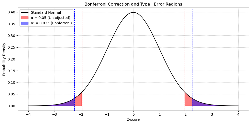
Interpreting the Diagram

**Bell curve showing original $\alpha$ and Bonferroni-corrected rejection regions.** The Bonferroni-adjusted regions lie farther from 0, reflecting the more stringent critical values.

The shaded areas represent rejection regions under two scenarios:

Outer shaded tails: Original $\alpha = 0.05$ rejection regions (2.5% in each tail)
Inner shaded tails: Bonferroni-adjusted $\alpha' = 0.025$ rejection regions (1.25% in each tail)

The critical value for Bonferroni (CVB) is the $t$- or $z$-value that corresponds to $\alpha'$, which lies further from 0 than the uncorrected critical value. This makes it harder to reject $H_0$.

Key Concepts Illustrated

Without correction: \[ P(\text{at least one TIE}) = 1 - (1 - \alpha)^K = 1 - (0.95)^2 = 0.0975 \]
With Bonferroni correction: \[ \alpha' = \frac{0.05}{2} = 0.025 \quad \Rightarrow \quad P(\text{at least one TIE}) = 1 - (0.975)^2 = 0.0494 \]
CVB (critical value for Bonferroni) moves farther from 0, tightening the rejection region.
Bonferroni maintains a familywise error rate at or below 0.05.

Summary

When we conduct multiple comparisons, the overall Type I error rate is inflated.
The Bonferroni correction addresses this by adjusting the per-comparison significance level: \[ \alpha' = \frac{\alpha}{K} \]
Pros:
- Simple and widely applicable
- Works for any number of tests
- Makes no assumptions about the test structure
- Can be applied directly to p-values
Cons:
- Can be overly conservative
- Reduces power, making it harder to reject $H_0$

Multiple Comparison Procedures — Handicap Study

We now explore multiple comparison questions using the Handicap study data. These comparisons build on the need for error rate control, such as the Bonferroni adjustment, after identifying overall group differences.

Questions of Interest (QOIs)

Are any pairs of group means different?
Does the Amputee group have a different mean score than the None group?
Which specific pairs of groups differ?
Do the means of the four Handicap groups differ from the Non-Handicap (None) group?

Each of these questions involves multiple comparisons and may require adjustment for familywise error rates.

QOI 1: Are Any Group Means Different?

We begin with an overall test to determine if there are any mean differences across the five groups. This involves an ANOVA and is the first step in any further group comparisons.

Assumptions:
- Normality
- Equal variances (e.g., visual checks and Brown–Forsythe test)
- Independence (assumed from study design)

Hypotheses: \[ H_0: \mu_1 = \mu_2 = \dots = \mu_5 \quad \text{(All group means are equal)} \] \[ H_A: \text{At least two group means differ} \]
Critical value: $F_{\alpha, 4, 65}$
ANOVA test statistic ($F$-statistic): $F = 2.85$
p-value: $p = 0.0301$
Decision: Reject $H_0$ (needle in the haystack)
Conclusion: There is sufficient evidence at $\alpha = 0.05$ to conclude that at least two group means differ ($p = 0.0301$, from a standard ANOVA).

Since the omnibus ANOVA test is significant, we proceed to investigate which group differences are driving the result. Multiple comparison procedures will be necessary to identify specific contrasts.

Model fitting R code (for context):

Code

fit <- aov(Score ~ Handicap, data = Handicap)

QOI 2: Does the Amputee Group Differ from the None Group?

We now test whether the mean score for the Amputee group differs from that of the None group.

This contrast was identified before looking at the data (i.e., a planned comparison), so we do not need to apply a multiple comparison correction.

Hypotheses:

\[ H_0: \mu_{\text{Amp}} = \mu_{\text{None}} \] \[ H_A: \mu_{\text{Amp}} \ne \mu_{\text{None}} \]

Options for Testing the Contrast:

We could use one of the following approaches:

Two-sample $t$-test (just Amputee vs. None):
- Pooled standard deviation
- Degrees of freedom: $df = 26$
- $t$-distribution
- $p$-value: 0.4678
Fit a GLM model using only Amputee and None:
- Equivalent $F$-statistic
- Same result as above: $df = 1$, $26$
- $F$-distribution
- $p$-value: 0.4678
Best option: Use all 70 observations:
- Use the pooled standard deviation from the full model
- Conduct the planned contrast within the global ANOVA model
- Critical value: $F_{, 4, 65}
- $F$-statistic with extended degrees of freedom: $df = 65$
- $p$-value: 0.4477

Conclusion:

Decision: Fail to reject $H_0$
Interpretation: There is not sufficient evidence to suggest that the mean rating of the Amputee group is different from the None group (p = 0.4477 from a contrast using all the data).

QOI 3: Which Specific Pairs of Groups Differ?

We now explore whether there is evidence that any specific pair of group means differ. These are not planned comparisons, so we must adjust for the increased chance of Type I error due to multiple testing.

There are 5 groups, which gives $K = \binom{5}{2} = 10$ pairwise comparisons.
Without correction, the risk of at least one false positive (rejecting $H_0$ when it is true) increases.
The Bonferroni correction provides a simple solution by adjusting the significance threshold.

Unadjusted Procedure
Compare each group pair using pairwise comparisons without correction:

Code

proc glm data=Handicap;
  class Handicap;
  model Score = Handicap;
  means Handicap / hovtest=bf;
  ls means Handicap / pdiff;
run;

Compare each pair’s raw p-value to $\alpha = 0.05$
Inflated Type I error risk due to multiple tests

Bonferroni Adjustment and Procedure:
To control the familywise error rate, adjust $\alpha$ using the Bonferroni correction:

Adjusted threshold: $\alpha' = \frac{\alpha}{K} = \frac{0.05}{10} = 0.005$
Use Bonferroni-adjusted confidence intervals and p-values to control the error rate across the family of comparisons.

The Bonferroni-adjusted analysis in SAS uses the adjust=bon option:

Code

proc glm data=Handicap;
  class Handicap;
  model Score = Handicap;
  means Handicap / hovtest=bf;
  ls means Handicap / pdiff adjust=bon cl; *cl = confidence level;
run;

The cl option provides Bonferroni-adjusted confidence intervals.
These intervals are wider because:
- $\alpha$’ is smaller than $\alpha$.
- The critical value is larger.
- The multiplier increases.
- Wider intervals result from a more conservative correction.
The cldiff option gives both directions (e.g., $A - B$ and $B - A$).
Each p-value is multiplied by $K$ before comparison to the original $\alpha$: \[ K \cdot p_{\text{adj}} \leq \alpha \]

Interpretation:

This procedure protects against Type I error across the entire family of tests.
It is conservative but appropriate when many unplanned comparisons are being made.

Conclusion:

After applying the Bonferroni adjustment,only 1 of the 10 tests produced a statistically significant result. Therefore, there is evidence (p-value = 0.0035 from a t-test) that the Crutches and Hearing groups have different mean ratings. A 95% Bonferroni-adjusted confidence interval for the difference in means between the Crutches and Hearing groups is $(0.0779,\ 3.6649)$.

QOI 4: Do the Means of the Four Handicap Groups Differ from the Non-Handicap (None) Group?

Assume we are interested in testing whether the means of the four handicap groups differ from the mean of the non-handicap group (i.e., the None group).

Use Dunnett’s procedure because we are comparing the control group (None) to all the others — a pairwise set of dependent comparisons (repeating the control group).

Option 1: Dunnett-adjusted confidence intervals

Specify the control group on the right side using dunnett('None')
Also provides Dunnett-corrected confidence intervals

Code

proc glm data=Handicap;
  class Handicap;
  model Score = Handicap;
  means Handicap / hovtest=bf dunnett('None');
run;

Option 2: Dunnett-adjusted p-values only

Use control('None') to specify the control group
Provides Dunnett-adjusted p-values for all pairwise comparisons with the None group

Code

proc glm data=Handicap;
  class Handicap;
  model Score = Handicap;
  ls means Handicap / pdiff=control('None');
run;