Objectives
- Calculate and interpret residuals, standardized residuals, and studentized residuals.
- Use residuals to check regression assumptions.
- Apply necessary remedies when assumptions are violated.
- Understand the robustness of assumptions (i.e., what can you get away with?)
Robustness of Regression Assumptions
Linearity
- Parameter estimates will be misleading if a straight-line model is inadequate or fits only part of the data.
- Predictions will be biased, and confidence intervals (CIs) will not appropriately reflect uncertainty.
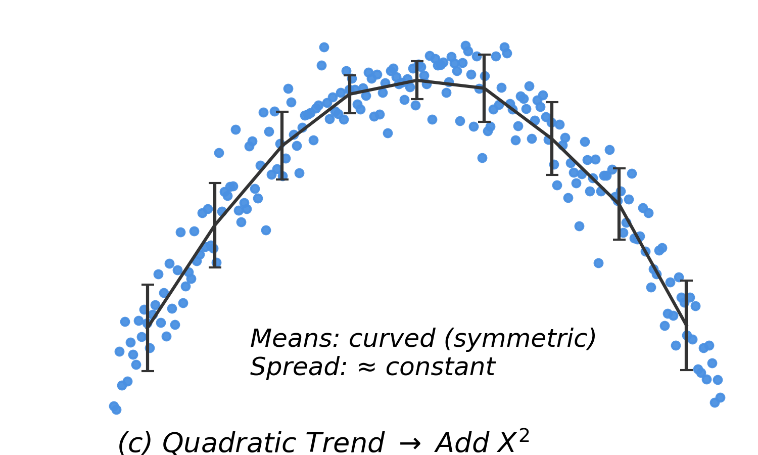
- Remedy: Consider adding polynomial terms (quadratic or cubic) to improve model fit.
Normality
- Transformations that correct for normality often address constant variance as well.
- Effects of non-normality:
- Coefficient estimates and standard errors: Robust, except with many outliers and small sample sizes.
- Confidence intervals: Affected primarily by outliers (long tails).
- Prediction intervals: Sensitive to non-normality due to reliance on normal distributions.
Constant Variance (Homoscedasticity)
- For every value of \(x\), the spread of \(y\) should be the same.
- Least squares estimates remain unbiased with slight violations.
- Large violations can cause standard errors to underestimate or overestimate uncertainty, leading to misleading confidence intervals and hypothesis tests.
- Remedy: Large violations should be corrected using a transformation.
Independence
- Parameter estimates: Not affected by violations.
- Standard errors: Affected significantly. Violations can lead to underestimated standard errors, which inflate t-statistics and make it easier to incorrectly reject the null hypothesis.
- Remedy: Serial and cluster effects require different models.
How Much Deviation Is Acceptable?
- Small violations of assumptions generally do not invalidate regression results.
- However, large deviations can lead to inaccurate estimates, especially for standard errors, confidence intervals, and p-values.
- Transformations can often correct violations and improve interpretability.
- Only severe departures from linearity or normality (e.g., due to outliers) typically require alternative methods.
Influential and Outlying Observations
Key Concepts
- Influential observations: These are points that, if added or removed, substantially change the regression line (e.g., the slope or intercept).
- Leverage: A measure of how far an observation’s \(x\) value is from the mean of all \(x\) values (\(\bar{x}\)).
- Points farther from \(\bar{x}\) have higher leverage.
- Mathematically, leverage increases with the squared distance from \(x_i\) to \(\bar{x}\), relative to the total sum of squares in \(x\). This is closely related to how many standard deviations \(x_i\) is from the mean.
- Leverage is based on the \(x\) values alone; it does not depend on \(y\).
Impact of Outliers
- Low leverage, low influence: Minimal effect on estimates.
- High leverage, low influence: Far from most data but consistent with the trend; minimal effect on the correlation, standard errors, and regression estimates.
- High leverage, high influence: Can distort results by pulling the regression line toward the outlier, resulting in different parameter estimates.
Detecting Influential Observations
Leverage Statistic, \(h_{ii}\)
- Measures how far the \(x\) value for an observation is from the mean \(\bar{x}\), in relation to the total spread of \(x\) values. Larger values of \(h_{ii}\) indicate higher leverage.
- An observation is considered to have high leverage if \(h_{ii} > \dfrac{2p}{n}\), where \(p\) is the number of parameters in the model (including the intercept).
- Formula: \[
h_{ii} = \frac{1}{n} + \frac{(X_i - \bar{X})^2}{\sum_{j=1}^{n} (X_j - \bar{X})^2}
\] or \[
h_{ii} = \frac{1}{n - 1} \left[ \frac{(X_i - \bar{X})}{s_x} \right]^2 + \frac{1}{n}
\]
Types of Residuals
- Standardized: \(e_i / \text{RMSE}\)
- Studentized: \(e_i / \sqrt{\text{MSE} \cdot (1 - h_{ii})}\)
- Studentized-deleted (R-student):
- Remove an observation, recalculate the regression, and compute the studentized residual.
- The standard deviation is calculated without the point in question.
- Large residual values indicate potentially influential points.
- Formula: \[
\text{RSTUDENT} = \frac{\text{res}_i}{s_i \sqrt{1 - h_i}}
\]
- Why different types? All three aim to stabilize variance so that residuals are comparable, but they differ in how they estimate the error term:
- Standardized: Uses a single overall RMSE.
- Studentized: Adjusts for leverage via \((1 - h_{ii})\).
- R-student: Recalculates without the observation for more accurate influence detection.
Leave-One-Out Statistics
These measures assess the impact of each observation by considering the model fit when that observation is omitted.
Let \(\hat{Y}_{i(i)}\) be the predicted value of \(Y_i\) when the \(i\)-th observation is left out of the regression model.
PRESS (Predicted Residual Sum of Squares)
\[
\text{PRESS}_p = \sum_{i=1}^n \left(Y_i - \hat{Y}_{i(i)}\right)^2 = \sum e_{i(i)}^2
\]
- Smaller PRESS values indicate better-fitting models.
Cook’s Distance (\(D_i\))
- Combines information on residual size and leverage, and is equivalent to comparing predictions from the full model to those from a leave-one-out model: \[
D_i = \sum_{i=1}^n \frac{\left(\hat{Y}_{i(i)} - \hat{Y}_i\right)^2}{p \cdot \text{MSE}} = \frac{1}{p} (\text{studres}_i)^2 \left[\frac{h_i}{1 - h_i}\right]
\]
- Here, \(p\) is the number of parameters in the model (including the intercept).
Durbin-Watson Test for Independence
\[
d = \frac{\sum_{i=1}^n (e_i - e_{i-1})^2}{\sum_{i=1}^n e_i^2}
\]
- Values near 0 indicate positive correlation; values near 4 indicate negative correlation. The distribution is symmetric about 2.
- Available in R and SAS.
Residual Types Summary
| Residual |
\(e_i = y_i - \hat{y}_i\) |
Residual plots |
| Standardized residual |
\(r_i = \frac{e_i}{s \sqrt{1 - h_{ii}}}\) |
Identify outliers |
| Studentized residual |
\(t_i = \frac{e_i}{s_{(i)} \sqrt{1 - h_{ii}}}\) |
Test outlying \(Y\) values |
| Deleted residual |
\(e_{i(i)} = y_i - \hat{y}_{i(i)} = \frac{e_i}{1 - h_{ii}}\) |
Calculate PRESS |
For studentized residuals, at \(\alpha = 0.05\) we expect about 5% to be greater than 2 or less than –2.
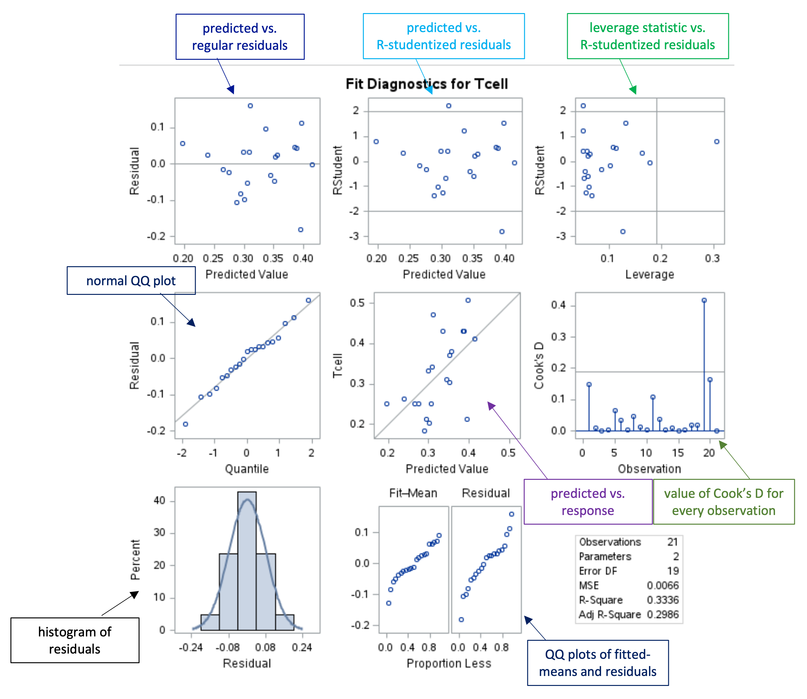
Residual Diagnostics Panel
Graphical Assessment of Residuals
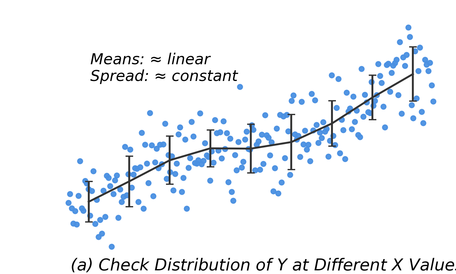
| Linear means, constant SD |
Model fits well |
No action needed |
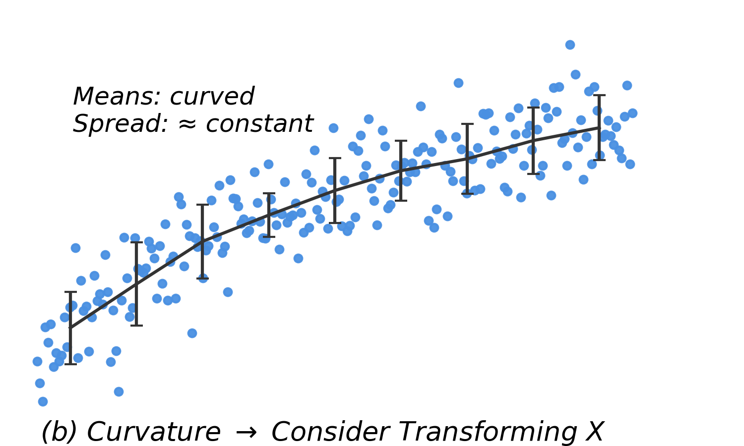
| Curved means, equal SD |
Nonlinearity |
Transform \(X\) |
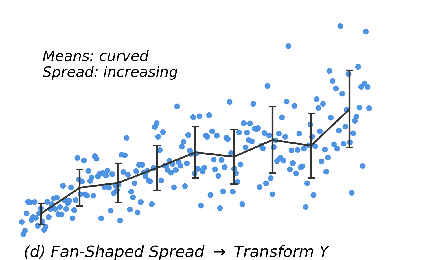
| Curved means, increasing SD |
Nonlinearity + heteroscedasticity |
Transform \(Y\) |
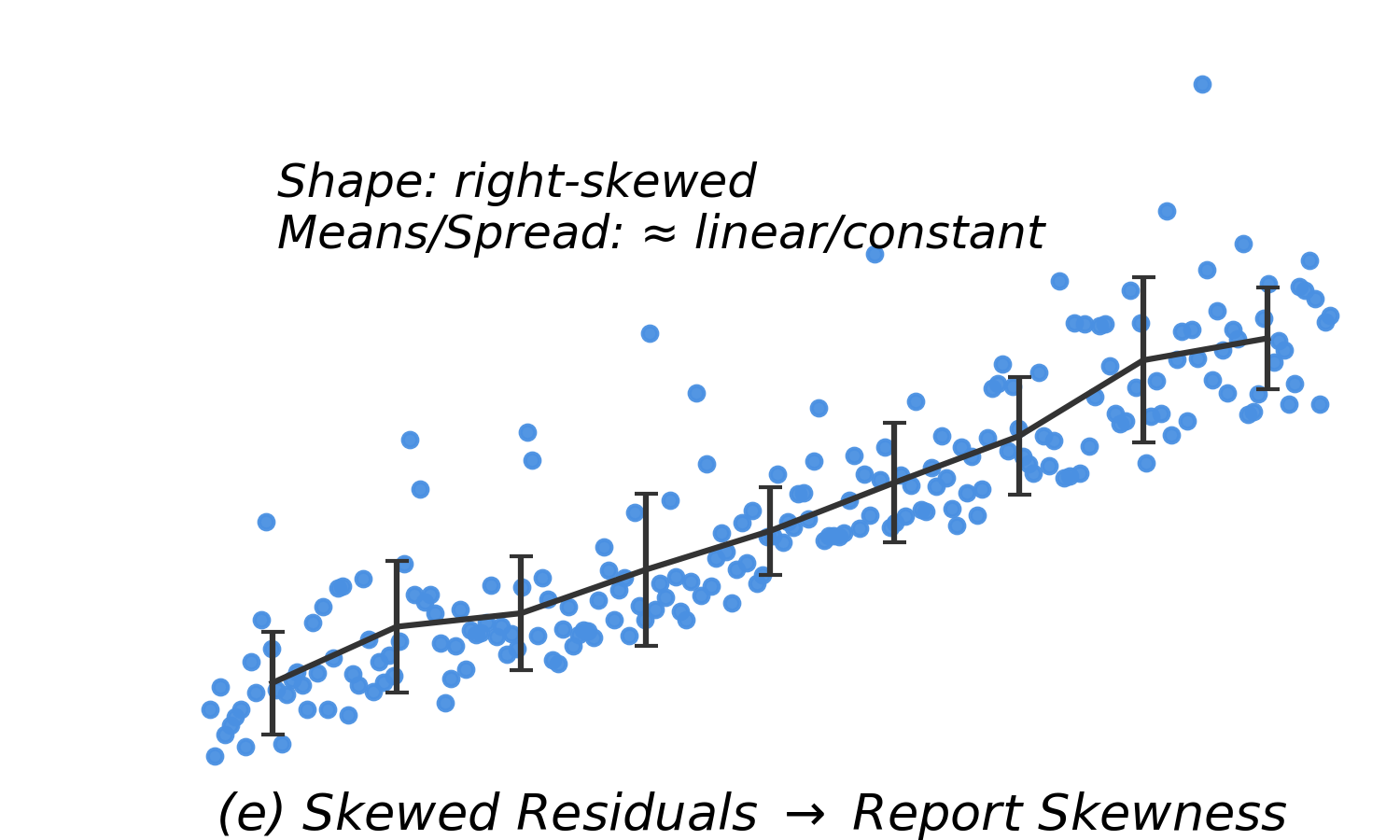
| Skewed residuals |
Non-normality |
Can still model the mean, but CIs/PIs may be unreliable. Consider transformations. |
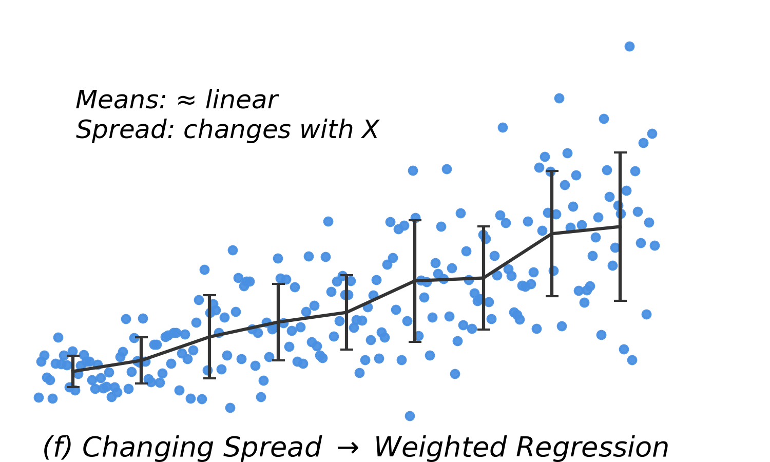
| Linear means, increasing SD |
Heteroscedasticity |
Use weighted regression |
Remedies for Violations
Nonlinearity
- Add more complexity to the model.
- Apply a transformation to \(X\).
- Add another variable, which may also help nonconstant variance.
Nonconstant Variance
- Transform \(Y\).
- Use weighted least squares to down-weight observations with larger variance so they don’t influence the regression model as much as observations closer to the line.
Outliers
- Use robust regression.
- Check for data entry or other errors. Only delect observations in this situation.
Non-normality
- Usually fixed via the above methods, so wait to fix until last.
- Consider transforming the data.
Residual Patterns and Suggested Remedies
Summary Table: Interpretation by Model Type
|
Model Type
|
Equation
|
Interpretation
|
|
Log-linear
|
\(\log Y = \beta_0 + \beta_1 X\)
|
1 unit increase in \(X\) \(\rightarrow\) \(e^{\beta_1}\) change in median \(Y\)
|
|
Linear-log
|
\(Y = \beta_0 + \beta_1 \log X\)
|
Doubling \(X\) \(\rightarrow\) \(\beta_1 \log(2)\) change in mean \(Y\)
|
|
Log-log
|
\(\log Y = \beta_0 + \beta_1 \log X\)
|
Doubling \(X\) \(\rightarrow\) ×\(2^{\beta_1}\) change in median \(Y\)
|
Note: Logging \(Y\) generally shifts interpretation from the mean to the median.